Background

Recently I’ve been diving into neural networks. After watching 3Blue1Brown’s neural network series (I highly recommend if you haven’t seen it), I was ready to dive into actually implementing one. But I quickly found that using Pytorch to train an MNIST model wasn’t too exciting after learning the nitty gritty of how neural nets work. I felt it was only necessary to try and train a model by implementing backpropagation from scratch, not only as a fun exercise but also to really reinforce my knowledge of neural networks.

This blog mainly serves as a guided walthrough for the math behind neural networks and then shares some hints for implementing one from scratch. I also include some of my experience and challenges I faced implementing a neural net. I’ll share minimal code and leave the implementation details as an exercise to the reader. Before following along, I would make sure your comfortable in these areas:

• Linear algebra (vector/matrix operations, especially dot products and matrix multiplication)
• Multivariable calculus (chain rule, gradients, Jacobians, matrix calculus)
• Probability rules and distributions
• Python and NumPy, or whatever language you decide to use.

Don’t worry if you don’t know multivariable calculus. I haven’t taken a course in it yet, but as long as you understand partial derivatives you’ll be fine. I’ll explain the relevant multivariable concepts, since that is really the hardest part of backpropagation anyway. But, you should definitely understand the linear algebra concepts. I’ll explain as if you have never heard of a neural network before. If you get stuck, my finished project is available on github, but I encourage you to try to work through it yourself.

These are the concepts we’ll cover in order:

• Neural network overview
• Forward pass
• Loading and handling data
• Using the network to make predictions
• Backward pass, including automatic differentiation
• Training the network
• Accuracy optimization

Neural Network?

Let’s first talk about what a neural network actually is. A neural network is a machine learning model inspired by neuroscience. It consists of a network of neurons and connections between them, taking some input data and making some prediction. In our case, we want to take image data and predict what digit is written inside the image.

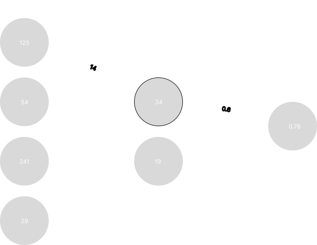
Each neuron has some value that can pretty much be any real number. This is called the activation value of the neuron. The connection between two neurons is also represented by some real number, and its value is called a weight, which basically represents the strength of the connection that affects the activation values of neurons. A bias value is also a added to the weight, and then a non-linear activation function is applied to get the final activation value for the neuron.

Our neural network will have a very specific architecture. It will contain layers of neurons in a very ordered way, with each layer fully connected to the previous and next layer. This means that each neuron will connect to every other neuron in the previous and next layer. Generally, the first layer will be an input layer (image data in our case), then there will be some number of hidden layers, and then an output layer with a prediction. The hidden layers are where all the magic of neural networks happen, which we will see later.

When we first create our neural network, it will have completely random weights, meaning that everything will be totally random and our prediction will be non-sense. Generally, it will predict around a 10% probability for each digit for any image you give it, even if that image contains no digit at all. We have to train our neural network to fine tune its weights so that its prediction is actually accurate, which will be our main goal.

Forward Pass

The forward pass of the network starts with the input image data, which is then passed through the hidden layers where neurons are activated based on the strength of all previous connections and the previous neuron activations. Let’s focus on how to compute an activation value for a single neuron.

Since the layers are fully connected, a single neuron will have connections from every neuron in the previous layer, which themselves have activation values, weights, and biases for the connection to this neuron in question. Right now our goal is to find the activation value for a single neuron in the second layer, that is the layer right after the input layer. This is the first layer whose activations we need to find, since the first layer is already given by the input.

Math

The activations, weights and biases are represented by vectors. Let $n$ be the number of neurons in the input layer, and $m$ be the number of neurons in the second layer. Our goal is to find the activation value for the ith neuron in the second layer. We’ll call the activation vector for the first layer $\mathbf{x}$, since it’s our input that does not need to be computed, and it has $n$ dimensions. To represent the weights, we’ll use another vector $\mathbf{w_i}$ (eventually will be part of a matrix, hence the subscript) where each component corrosponds to a connection from the corrosponding neuron in $\mathbf{x}$ to this ith neuron, so it is also n-dimensional. Finally, $b_i$ is a scalar that represents the bias for this neuron.

To find the activation for a single neuron, we’ll take the weighted sum of all neuron activation values from the previous layer weighted by their weights, then add the bias for the neuron to it. So let’s say we want to find $z_i$, which is an intermediate value of the activation for the ith neuron. Then, $z_i = \mathbf{w_i} \cdot \mathbf{x} + b_i$. The dot product naturally represents the weighted sum, and then we just add a scalar bias to it. Then to get the actual activation $a_i$, we apply some non-linear activation function $f(x)$ to $z_i$, so $a_i = f(z_i)$. This is necessary so that we introduce non-linearity to the network. Without it, we could only capture linear transformations, which would significantly limit what it could do. I put the definitions of the functions we need at the bottom of this section so you don’t get bogged down by them for now.

Now that we can find the activation for a single neuron in the second layer, this idea naturally scales up to allow us to find every neuron activation in the second layer, with a few additions. We need to create a matrix $W$ that contains information on all of the weights for each neuron. But what dimensions will it have? This confused me when implementing my neural network, so it’s worth mentioning here. Remember, $w_i$ is part of this matrix, and specifically it is the ith row of it. So, we need $m$ rows, since i is tracking the neuron in the second layer, and we have $m$ neurons in the second layer. And each row vector in $W$ will need to be $n$ dimensional, since $w_i$ was $n$-dimensional.

$$W = \begin{bmatrix} w_1 \\ w_2 \\ w_3 \\ \vdots \\ w_m \end{bmatrix} \implies W = \begin{bmatrix} w_{1,1} & w_{1,2} & \dots & w_{1, n} \\ w_{2,1} & w_{2,2} & \dots & w_{2, n} \\ w_{3,1} & w_{3,2} & \dots & w_{3, n} \\ \vdots & \vdots & \ddots & \vdots \\ w_{m, 1} & w_{m, 2} & \dots & w_{m, n} \end{bmatrix}$$

To find $\mathbf{z}$, which represents the vector of all intermediate activation values of the second layer, we do a similar calculation that we did to find $z_i$. But, instead of using the dot product, we need to do matrix multiplication, since it is basically a scaled up dot product. And now we also use a vector $\mathbf{b}$, which represents the biases of all the neurons in the second layer. So, $\mathbf{z} = W\mathbf{x} + \mathbf{b}$, which is basically just a compact way to do what we did with the single neuron to every neuron at once. After we have the intermediate activation, we then get the actual activation vector with $\mathbf{a} = f(\mathbf{z})$, where $f$ is just applied to each element in $\mathbf{z}$.

Now that we can find the activation for the second layer, the activation for the next layers are the same, except instead of using $\mathbf{x}$, we just use the previous activation vector of the last layer to find the current one. It’s helpful to index the activation and pre-activation values for each layer with a superscript to represent which layer it’s in. We’ll start at zero, so the first input layer activation vector will be represented as $\mathbf{a^{(0)}}$ (note this is not an exponent) since we want the first layer activation vector, then $w^{(1)}$ represents the weight matrix for the first layer, and $\mathbf{b^{(1)}}$ for the biases of the first layer. Then, to find $\mathbf{a^{(1)}}$, which is the activation for the second layer, first we need $\mathbf{z^{(1)}}$, the pre-activation for the second layer. Same math as before, just being explicit about which layer we’re getting things from. So, $\mathbf{z^{(1)}} = W^{(1)}\mathbf{a^{(0)}} + \mathbf{b^{(1)}}$. Then just like before, $\mathbf{a^{(1)}} = f(\mathbf{z^{(1)}})$, using some non-linear activation function $f$ which I explain in the next part.

Make sure that you really understand the math of the forward pass before moving on. It can be intimidating because there is a lot going on, so read this section a few more times if needed.

Activation Functions

The most common activation function is ReLU, which stands for rectified linear unit. It’s a piecewise linear function defined as:

$$ReLU(z_i) = \begin{cases} z_i & \text{if } z_i > 0 \\ 0 & \text{otherwise} \end{cases}$$

So if the pre-activiation $z_i$ is negative, it’s activated value will just be zero. If it’s zero or positive, it won’t change. It’s used because it’s very easy to compute, yet it gives us non-linearity. We’ll use this function for all the hidden layers, which are the layers in between the first and last layer.

For the last layer, we’ll use the softmax activation function. We want our output layer to be a probability distribution where all the final neurons sum to one. Each individual neuron tells us the predicted probability that our input image is an image of the corrosponding digit. Softmax will turn our final pre-activation layer into this probability distribution. For example, if the output activation vector is $[0, 0, 0.9, 0, 0, 0, 0, 0.1, 0, 0]$, then the model is 90% confident the input image is a 2, and 10% confident it’s a 7. Here’s the definition:

$$S(z_i) = \frac{e^{z_i}}{\sum_{j=1}^k e^{z_j}}$$

Breaking it down, $z_i$ represents a pre-activation scalar value. We take $e$ and raise it to $z_i$, then divide it by the sum of $e$ raised to all of the pre-activation values for this layer. It’s basically like a regular probability with everything exponentiated.

Implementation

Now that we know how to do the forward pass, let’s try to implement the architecture of our neural network and perform a forward pass. This is the part where you can get creative, but I’ll share my implementation design for inspiration. And remember, we haven’t talked about actually training the network at all yet. Our goal for this section is to take our input data and get an output that predicts that the probability that our input is a specific digit, and we expect around a 10% probability for each digit, since it has no idea what it’s doing yet.

First, we need a way to represent all of the parameters (weights and biases) of our network. For this, I created a NeuralNetwork class that will encapsulate all of the parameters of the network, and will include the forward pass behavior. I’ll be using NumPy to represent the vectors and matrices, but you can use whatever you want and even implement a tensor library from scratch if you want to. But instead of storing the parameters directly inside this class, it is also helpful to create another class for a layer in our network, that way we can encapsulate the data and behavior of an individual layer easily. I created a Layer class that takes the size of the input, output, and an activation function that will be used. At this point it would also be a good idea to define the ReLU activation function. All the layers except for the final output layer will use the ReLU activation function, then for the final layer we use softmax, so we also need to define the softmax function.

Inside of the Layer class, which has an input and output dimension, I created two members for the weights and biases of this layer, both initialized with the np.random.rand() function, which takes in the dimensions of the tensor. Refer back to the math section if you need help with determining the dimensions of these tensors with respect to the input and output size of the layer. The input size is just the size of the previous layer, and the ouput size is the number of neurons in this layer.

So far, you could have something with this outline:

def ReLU(x):
    ...

def softmax(x):
    ...

class Layer:
    def __init__(
        self, input_size,output_size, activation_func
    ):
        self.weights = np.random.rand(...)
        self.biases = np.random.rand(...)
        ...
    
    def forward(self, x):
        ...

class NeuralNetwork:
    def __init__(self):
        self.layers = [
            Layer(...),
            Layer(...),
            Layer(...)
        ]
    
    def forward(self, x):
        ...

Now we want to implement the forward pass for the Layer, which should return the activation vector after an input x has passed through the layer. This will involve calculating the pre-activation vector $\mathbf{z}$, then applying the activation function and returning the result.

Then, to implement the forward pass for the network, all we have to do is take our initial input x, feed it through the first layer, take the result of that and feed it to the next layer, and so on, until we reach the final output of the last layer. If you used a list like I did, it should be relatively easy to implement this.

Data Handling and Testing

Now we’ll use the neural network we’ve created and test it on the MNIST data set. Our goal is to evaluate the accuracy and get a result around 10%, since we haven’t trained it at all yet. All we’re doing is testing to make sure our input layer flows through the network correctly and gives us a valid output distribution.

To start, you’ll need to decide how to get the MNIST data. The easy route is to just use Tensorflow, Pytorch, or Scikit-learn to import it. But since we’re building the network from scratch, it felt right for me to parse the actual data set by hand, so I’ll explain how to do that. First, download the raw dataset from Kaggle here by downloading all the files ending in .idx3-ubyte and .idx1-ubyte.

Next, we’ll create the main program that parses the data, creates a NeuralNetwork object, and tests the accuracy of the forward pass. The MNIST data set is split into test and training files, both containing a separate file for the image data and labels. First, open the image training file in binary mode, and read the first 16 bytes for the file’s metadata. Byte 4-8 gives the number of images in the file, which we can extract using struct.unpack from the struct module

_, n_items, _, _ = struct.unpack(">iiii", f.read(16))

Then you can use the np.frombuffer function to read the images into a flat array, and then reshape it into a 2D tensor so that each image has it’s own row. The process is similar for the labels, you just read 8 bytes for the metadata instead of 16, and the number of labels is bytes 4-8, no re-shaping needed.

Once you have the images and labels in tensors, we can start doing the forward pass on the neural network and testing its accuracy. For now, we can just iterate over all the test images, put each one through the forward pass of the network, and see if it was correct based on the label. Remember, the output of the forward pass should be 10 neurons, each containg the probability the network thinks that the given image is of that corrosponding digit. We’ll say the network was correct if the neuron with the highest activation in the output matches with its labeled digit. So for example, if the last neuron in the output was 0.9, then the network would be 90% confident the given input was an image of a 9. And if the actual label is 9, then we mark it as correct. If it is something else, we’ll mark it as incorrect. Once you have the total correct and incorrect counts, calculate the accuracy. If your network is working so far, you should get a value around 10%, not significantly greater or worse than chance. If you aren’t getting near 10%, make sure your forward pass math is working correctly, and make sure the images and labels are being loaded and parsed correctly.

Now, our main program could look something like this:

def main():
    nn = NeuralNetwork()
    train_images, train_labels = load_mnist(...)

    correct = incorrect = 0
    for image, label in zip(train_images, train_labels):
        prediction = nn.forward(image)
        # decide if prediction is correct or not
        ...
    
    accuracy = correct / (incorrect + correct) 

Backward Pass

Now on to what I think is the most challenging part: the backward pass. The math in this section is genuinely difficult compared to the forward pass, so don’t feel bad if you need to re-read it multiple times. It took me at least 5x longer to understand the backward pass compared to the forward pass.

The backward pass happens after a forward pass. We calculate the loss of the prediction (how wrong the model was) based on a loss function, and then use this loss to find the gradient with respect to the weights and biases of the network. We then adjust the weights and biases accordingly to minimize the loss incurred from this forward pass by the training example. This algorithm is called backpropagation.

Essentially, the backward pass is how we actually train the model to fine tune its parameters so that we can create something actually useful that makes accurate predictions. At the end of this section, we should have a model that can predict a handwritten digit to at least 95% accuracy.

Math

First, let’s talk about the loss function. When we make a prediction from a forward pass, we need a way to tell the model how wrong it was. Say that the model predicts a 99% probability that the handwritten digit is a 0, so the final output neurons have .99 for the first neuron and then the remaing .01 will be distributed by the rest of the neurons. But, let’s say that the actual labeled digit is 8, so the labeled distribution has 1 for the 9th neuron and 0 for all the others (this is called “one-hot” encoding). Because the distributions are so different, and the model was confidently wrong, we want to “punish” the model quite harshly. For that, we use the cross entropy loss function. It is defined as:

$$L(\mathbf{y}, \mathbf{\hat{y}}) = -\sum_{c=1}^{C}y_c\log(\hat{y_c})$$

What does any of this mean? Well, $C$ is the number of classes, and we have 10 classes, each representing a digit. $y_c$ represents the $c$th element in the $\mathbf{y}$ vector, which is the labeled probability distribution. And $\hat{y_c}$ represents the $c$th element in the prediced probability distribution. So it takes the sum of the products of all the corrosponding elements in each distribution, just with a log applied to the labeled probability distribution. Kind of like a dot product! The log just punishes confident incorrect answers more.

We want to reduce the value of the loss by finding the optimal changes to the inputs that affect it. But what inputs affect it? As written, it looks like just $\mathbf{y}$ and $\mathbf{\hat{y}}$. But remember how we found $\mathbf{\hat{y}}$? It’s all the math that was done in the forward pass. All of the weights and biases of every layer affects $\mathbf{\hat{y}}$. So our goal with backpropagation is to go backwards through the network, and update the weights and biases in the most optimal way to most quickly reduce the value of the loss. Imagine this loss function is some surface in a space that is thousands of dimensions. Kind of hard to imagine, right? So instead, think of a surface in 3D. The surface has topography, and at any point on the surface, there is some direction to travel that leads to the quickest change in elevation.

The gradient is the vector that tells us which direction to move that leads to the fastest increase in the surface elevation. But we actually want the fastest decrease, because the elevation represents the loss or cost, which we want to minimize. So we’ll update the weights and biases based on the gradient in a process called gradient descent. This same idea translates to our thousands of dimensional space that has a dimensions for every single weight and biases.

Backpropagation

The algorithm we will use to find the gradient is backpropagation. We want to start from the last layer of the network, find it’s gradient with respects to the weights, and then find it’s gradient with respect to its biases. We’ll then use that information to update the weights and biases, and move back to the next layer and repeat until we get to the first layer. This is why it’s called the backward pass.

In my neural network, I have three layers, so the last one’s activation vector will be $\mathbf{a^{(2)}}$, weight matrix $W^{(2)}$, biases $\mathbf{b}^{(2)}$, and pre-activation $\mathbf{z^{(2)}}$. We want to find $\frac{\partial L}{\partial W^{(2)}}$, which is the gradient of the loss with respect to the third layers weights. This confused me, but even though this isn’t a vector, it’s the gradient. Each element in this matrix represents the amount that the corrosponding weight in the third layer needs to be adjusted for the fastest decrease in $L$. I didn’t know this at first, but it’s pretty simple:

$$\frac{\partial L}{\partial W^{(2)}} = \begin{bmatrix} \frac{\partial L}{\partial W_{1,1}^{(2)}} & \frac{\partial L}{\partial W_{1,2}^{(2)}} & \dots & \frac{\partial L}{\partial W_{1,n}^{(2)}} \\ \frac{\partial L}{\partial W_{2,1}^{(2)}} & \frac{\partial L}{\partial W_{2,2}^{(2)}} & \dots & \frac{\partial L}{\partial W_{2,n}^{(2)}} \\ \vdots & \vdots & \ddots & \vdots \\ \frac{\partial L}{\partial W_{m,1}^{(2)}} & \frac{\partial L}{\partial W_{m,2}^{(2)}} & \dots & \frac{\partial L}{\partial W_{m,n}^{(2)}} \\ \end{bmatrix}$$

It’s very important to understand the dimensions of all the matrices and vectors now. The biggest headache I encountered in the backward pass was dimensions not aligning for matrix multiplication. Save yourself a few hours and write them out.

So how do we find $\frac{\partial L}{\partial W^{(2)}}$? Remember, in the expression for L, we have $\mathbf{\hat{y}}$, not $w^{(2)}$. The key insight for me was that $\mathbf{\hat{y}}$ is really a long composition of functions, going all the way back to the first layer. We need to work backwards in this composition until we hit the expression involving $W^{(2)}$. To start, $\mathbf{\hat{y}}$ is really just $\mathbf{a^{(2)}}$, and $\mathbf{a^{(2)}} = S(\mathbf{z^{(2)}})$, where S is softmax. Then, $\mathbf{z^{(2)}} = W^{(2)}\mathbf{a^{(1)}} + \mathbf{b^{(2)}}$. And boom, just like that we found $W^{(2)}$, so we stop there.

Now this is where the chain rule comes in. You should understand the single variable case in this notation, which sometimes gets neglected:

$$\begin{align*} & y = f(u), \quad & u = g(x) \\ \\ & \frac{dy}{dx} = \frac{dy}{du} \frac{du}{dx} \end{align*}$$

We’ll use this notation because the function composition would get very messy. But, the loss function we’re dealing with depends on thousands of variables, so we’ll use partial derivatives instead of total derivatives. Remember, $\mathbf{\hat{y}}$ is what’s in the loss function, but that is the same as $\mathbf{a^{(2)}}$. So, all the compositions written out:

$$\begin{align*} & L = -\sum_{c=1}^{C}y_c\log(a^{(2)}_c) \\ \\ & \mathbf{a^{(2)}} = S(\mathbf{z^{(2)}}) \\ \\ & \mathbf{z^{(2)}} = W^{(2)}\mathbf{a^{(1)}} + \mathbf{b^{(2)}} \end{align*}$$

Now, using the chain rule, we need to keep finding derivatives until we reach $W^{(2)}$, so the derivative of L with respect to $W^{(2)}$ is:

$$\frac{\partial L}{\partial W^{(2)}} = \frac{\partial L}{\partial \mathbf{a^{(2)}}}\frac{\partial \mathbf{a^{(2)}}}{\partial \mathbf{z^{(2)}}}\frac{\partial \mathbf{z^{(2)}}}{\partial W^{(2)}}$$

If you’ve made it this far, then you basically understand the core idea of backpropagation. We’ll worry about the exact derivatives soon. But, the expression is very similar for finding $\frac{\partial L}{\partial W^{(1)}}$. See if you can find the composition continuing from the last layer and derive it yourself. Check your work:

$$\begin{align*} & \mathbf{a^{(1)}} = ReLU(\mathbf{z^{(1)}}) \\ \\ & \mathbf{z^{(1)}} = W^{(1)}\mathbf{a^{(0)}} + \mathbf{b^{(1)}} \\ \\ & \frac{\partial L}{\partial W^{(1)}} = \frac{\partial L}{\partial \mathbf{a^{(2)}}}\frac{\partial \mathbf{a^{(2)}}}{\partial \mathbf{z^{(2)}}}\frac{\partial \mathbf{z^{(2)}}}{\partial \mathbf{a^{(1)}}}\frac{\partial \mathbf{a^{(1)}}}{\partial \mathbf{z^{(1)}}}\frac{\partial \mathbf{z^{(1)}}}{\partial W^{(1)}} \end{align*}$$

That looks pretty messy. But do you notice anything? It looks like $\frac{\partial L}{\partial W^{(2)}}$ is almost included inside of $\frac{\partial L}{\partial W^{(1)}}$. It starts with $\frac{\partial L}{\partial \mathbf{a^{(2)}}}\frac{\partial \mathbf{a^{(2)}}}{\partial \mathbf{z^{(2)}}}$, just like $\frac{\partial L}{\partial W^{(2)}}$, but diverges with the next derivative, $\frac{\partial \mathbf{z^{(2)}}}{\partial \mathbf{a^{(1)}}}$. But because it’s so close, the idea is that we can just compute the derivative for each layer individually as long as we are given the slightly modified derivative from the previous layer.

So for every layer, we compute two separate derivatives. The first one is the actual gradient for the layer, $\frac{\partial L}{\partial \mathbf{a^{(2)}}}$. The next one will be the slightly modified derivative that, instead of having the $\frac{\partial \mathbf{z^{(2)}}}{\partial \mathbf{W^{(2)}}}$ term, contains the $\frac{\partial \mathbf{z^{(2)}}}{\partial \mathbf{a^{(1)}}}$ term. That derivative is $\frac{\partial L}{\partial \mathbf{a^{(1)}}}$. We’ll compute this one for efficiency, so that for each layer, instead of needing to compute all the previous layer’s derivatives, we can just use the previous layer’s derivative. This also easily allows us to just add a backward method to our layer. So each layer only needs to know it’s own derivative and the value of the modified derivative for the previous layer.

Now, let’s actually find the derivatives for just the last layer. I’ll work through step by step assuming you aren’t comfortable with multivariable differentiation, but feel free to gloss over the details if you are:

$$\frac{\partial L}{\partial a^{(2)}} = -\frac{\mathbf{y}}{\mathbf{a^{(2)}}} \\ \\$$

To find $\frac{\partial a^{(2)}}{\partial z^{(2)}}$, remember the full expression for $\mathbf{a^{(2)}}$:

$$\begin{align*} \mathbf{a^{(2)}} &= \frac{e^{z_i}}{\sum_{j=0}^{|\mathbf{z}|} e^{z_j}} \\ \\ \frac{\partial a^{(2)}}{\partial z^{(2)}} &= \frac{(\sum_{j=0}^{|\mathbf{z}|} e^{z_j})(z_i e^{z_i}) - (e^{z_i})(\mathbf{1})}{(\sum_{j=0}^{|\mathbf{z}|} e^{z_j})^2} \\ \\ &= \frac{z_i e^{z_i} - e^{z_i}}{\sum_{j=0}^{|\mathbf{z}|} e^{z_j}} \\ \\ &= \end{align*}$$